Category Archives: Statistical programming

Ninety years of rain

(Cross-posted from Kayak Yak Yak)

And some Novembers, that’s just the way it feels.

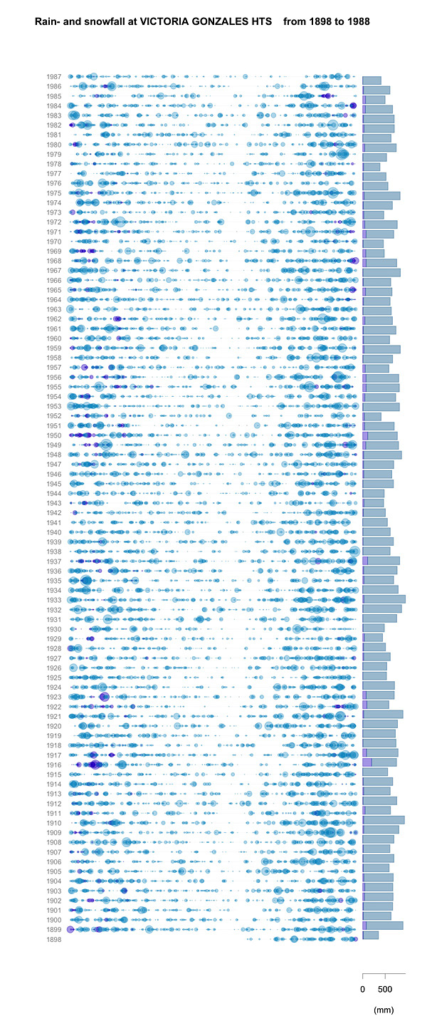
Inspired by this graphic, I have been playing around with the Canadian Daily Climate Data, available from Environment Canada National Climate Data and Information Archive. I’ll leave all the delightful geeky details of Python script and R code for another place and another time, but I wanted to show off my version of the plot, for the weather station at Gonzalez Heights (1898 to beginning of 1988). The area of the coloured circles are proportional to the rainfall, plotted per day along the horizontal and by year on the vertical (the San Francisco plot goes from mid-year to mid-year; mine currently uses the calendar year). On the right, the bars represent the total yearly precipitation. Rainfall is turquoise, snowfall is purple; snowfall is its liquid equivalent, not its snowy depth. During this period, the snowiest year was 1916 (199.4 mm by my calculation), with a one-day maximum of 53.3 mm (also in 1916). The rainiest year was 1933 (923.5 mm), although the maximum rainfall was 83.3 mm in 1979. Victoria International Airport has data from 1940 to 2004. None of these years (even 1996) was snowier, although the maximum snowfall, in 1996 (we know when that was!) was 64.5 mm. However the rainiest year was 1997, with 1159 mm, and the rainiest single day was in 2003, with 136 mm.

Precipitation at Gonzalez Heights weather station, Victoria

Shading between curves in R

As a R learner programmer, it took me unconscionably long to work out how to use polygon to shade under and between curves, despite searches of the R manual and R-help – they just didn’t start far enough back. So, for anyone else scratching his or her head over polygon (and so I can find it again when I forget how it’s done), here are the series of steps I went through to figure it out.

The function takes in an x vector and a y vector, defining a set of coordinates that, in order, taken in order trace around the area to be shaded. Thus for a set of points 1-10, defined individually as x.1, y.1 to x.10, y.10,

x <- c(x.1,x.2,x.3,x.4,x.5,x.6,x.7,x.8,x.9,x.10)
y <- c(y.1,y.2,y.3,y.4,y.5,y.6,y.7,y.8,x.9,y.10)

The area inside these points is shaded by

polygon(x,y,col=gray(0.8))

To apply this to two curves, both normal distributions between -3 and 3, one half the height of the other

x <- seq(-3,3,0.01)
y1 <- dnorm(x,0,1)
y2 <- 0.5*dnorm(x,0,1)
plot(x,y1,type="l",bty="L",xlab="X",ylab="dnorm(X)")
points(x,y2,type="l",col="red")
polygon(c(x,rev(x)),c(y2,rev(y1)),col="skyblue")

The first half of the x-vector in the polygon is just the values of x itself, corresponding to the part of the polygon that is tracing out the upper curve along increasing values of x. The second part for of the x-vector in the polygon is the reverse of x, corresponding to the part of the polygon that is tracing out the lower curve along decreasing values of x. The first part of the y-vector is the y values of the upper curve, and the second part of the y-vector is the y values of the lower part of the curve.

That shaded the area between the curves along the full plotted range.

To shade only a defined portion, say the area from x=-2 to x=1.

x <- seq(-3,3,0.01)
y1 <- dnorm(x,0,1)
y2 <- 0.5*dnorm(x,0,1)
x.shade <- seq(-2,1,0.01)
polygon(c(x.shade,rev(x.shade)),c(dnorm(x.shade,0,1),0.5*dnorm(rev(x.shade),0,1)),col="yellow")

To shade the same defined portion as a gradient, from red to yellow (from the built-in heat.colors palette):

x <- seq(-3,3,0.01)
y1 <- dnorm(x,0,1)
y2 <- 0.5*dnorm(x,0,1)
x.shade <- seq(-2,1,0.01)
par(oma=c(1,1,1,1),cex=0.7)
plot(x,y1,type="l",bty="L",xlab="X",ylab="dnorm(X)")
points(x,y2,type="l",col="gray")
l <- length(x.shade)
color <- heat.colors(l)
for (i in 1:l)
{
polygon(c(x.shade[i],rev(x.shade[i])),c(dnorm(x.shade[i],0,1),
0.5*dnorm(rev(x.shade[i]),0,1)),border=color[i],col=NA)
}

This draws a succession of individual polygons between the curves, adjusting the color along the gradient as it goes. (Note that the loop above is for i in one to letter-L).

A few of my favourite tools: Wine

Wine (named in recursive fashion “Wine is not an emulator”) is used to run Windows applications on Linux; essentially, it interprets Windows commands for Linux and vice versa. I first met Wine in the form of Darwine (the “Dar” being for the underlying Darwin windowing technology in OSX), ported and maintained by Mike Kroneberg, and described at Low End Mac in an article by Alan Zisman. An alternative approach to installing wine, which I have not explored, is to install Wine via MacPorts.

The utility of Wine is that it does not require one to partition the hard drive, reboot, or to own and run any version of Windows. I have a full installation of Windows Vista Pro running on Parallels, but for certain lightweight, self-contained programs, I can launch Darwine and be running in a quarter of the time it takes for Parallels and then Vista to lumber into motion. WinBUGS, which I’ve been learning for Bayesian analysis, runs quite happily on Darwine, although I had to install by downloading and unpacking a zip file (per instructions for Vista or 64 bit systems), as the installer itself gave an error. After that, about the only tricky part was figuring out the file structure of the pseudo-C drive and how to access the files on the Mac, since they’re in an invisible folder. FirstBayes (Bayesian learning software) did not run, even after I figured out how to do the required registry hack, but then FirstBayes didn’t care much for Vista, either. Notepad++ runs without any trouble, as does Plant Studio (an old Windows program for building 3D plant models). Here is the official application database, rather games-heavy.

Darwine is no longer being developed, but its successor, now named Wine, is still in development. As my copy of Darwine survived beyond the Snow Leopard Event Horizon and still does what I need it to do, I will upgrade later.